Connect without Contact
Our magnetic sensors provide accurate and reliable data – without physical contact.
Sensors that monitor properties such as temperature, pressure, strain or flow provide an output signal that is directly related to the desired parameter. Magnetic sensors, on the other hand, differ from most of these detectors as they very often do not directly measure the physical property of interest. They detect changes, or disturbances in magnetic fields that have been created or modified by objects or events. The magnetic fields may therefore carry information on properties such as direction, presence, rotation, angle, or electrical currents that is converted into an electrical voltage by the magnetic sensor. The minor amount of magnetic sensors measure magnetic fields absolutely, like earth field in compassing.
The output signal requires some signal processing for translation into the desired parameter. Obviously, a magnetic field distribution depends on distance and the form of the creating or disturbing object (i.e., magnet, current, etc.) or event. It is therefore important always to consider both sensor and creating object in the application design. Although magnetic sensors are somewhat more difficult to use, they do provide accurate and reliable data — without physical contact.

MAGNETORESISTIVE EFFECT
History
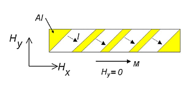
Lord Kelvin discovered magnetoresistance in 1857 when he noticed the slight change in the electrical resistance of a piece of iron when he placed it in a magnetic field. But it took more than 100 years before a first magnetoresisitve (MR) sensor concept was reported by Hunt in 1971. And it lasted additional 20 years for IBM to introduce the first MR head, which used a strip of magnetoresistive material to detect bits, into a hard disk drive in 1991. Earlier, MR sensors were used in less demanding applications of price-tag and badge readers (read-only) and magnetic tape (1985). The geometry of a Hunt element – a magnetoresistive film with a sense current I and magnetization vector M at a signal determining angel α to the current in the plane of the film (see Figure 1). A magnetic field Hy coupled into the soft magnetic sensor material will change the resisitivity of the stripe, which is probed by the sense current.

Figure 1: The geometry of a Hunt element
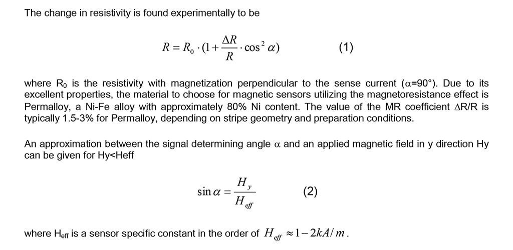
The physical origin of the magnetoresistance effect in the transition metals lies in the dependence on the direction of the magnetization of the scattering of electrons. In the transition metals, the predominant carriers of current are the 4s electrons since they have a higher mobility than the 3d electrons. The scattering of electrons from the s to the d bands is found to be highest when the electrons are travelling parallel to the magnetization.
Wheatstone Bridges
In most applications, the academic Hunt element is not suited as it does not provide a zero reference. This disadvantage as well as the temperature dependence of the resistance can be avoided by using a Wheatstone bridge.
Magnetic Units
A fairly confusing situation on magnetic units appears to the normal reader, who is not a specialist in magnetism. The following table shall help to find conversion factos quickly between the different units used:
| Unit 1 | Multiply By | = Unit 2 | Remark |
|---|---|---|---|
| Tesla | 104 | Gauss | |
| Oerstedt |
1 | Gauss | μr = 1 ! |
| Oerstedt | 79.58 | A/m | 103/(4xπ) |
| Weber | 108 | Maxwell |
Table 1: Conversion factors for magnetic units; for detailed information, refer to the NIST homepage.

MAGNETORESISTIVE SENSORS
Sensor Types by Magnetic Field
Magnetoresistive sensors can basically be divided into two groups. In high field applications, such as where the field strength of the applied field is strong enough to saturate the soft magnetic sensor material (roughly for H>10 kA/m), the magnetization vector in the sensor is always (almost) parallel to the applied field. A common application for a magnetoresistive high field sensor is a contactless angular sensor, like the KMT32B, the KMT36H or the MLS-position sensors. In low field applications the magnetization vector is mainly determined by the form of the strips, because the magnetization shows a natural preference for the longitudinal direction. The external field causes a twist α of the magnetization in the stripe, which changes the resistance due to the MR effect. Linear low field sensors like the MR174B die, the KMY sensors and switching sensors like the MS32 are typically working in this mode.
MR Sensors
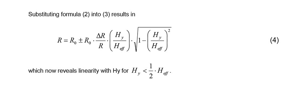
With Linearized Transfer Curve
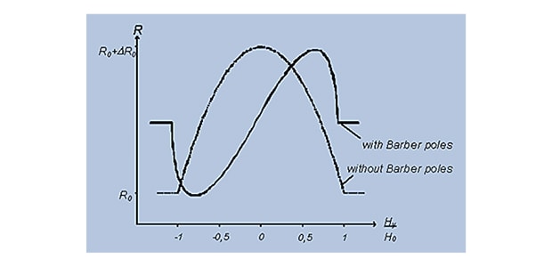
Applying low magnetic fields to a Hunt element will lead only to small changes of the magnetization and in turn, the cos term in formula (1) will hardly change at small changes of α. A Hunt element is not sensitive at small field strengths. In order to make the MR sensor sensitive for low magentic fields, the MR transfer curve (1) has to be modified. The most common way is achieved by barber poles (see Figure 2.)
Small, highly conductive bars – the barber poles – are placed on top of the Permalloy. They will shunt the current in the Permalloy and will change the current path due to their geometry, but they will not change the magnetic behavior. The current between the barber pole gaps will take the shortest path, such as perpendicular to the barber poles.
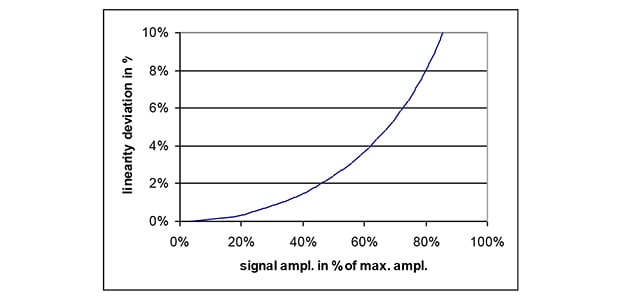
Sensor Linearity
The linearity of the sensor output signal depends on the relation of the real signal amplitude to the maximum output voltage amplitude. Figure 4 shows the linearity deviation in relation to this quotient (in percent):
Sensor Stability
The magnetostatic energy is the same for a magnetic domain whether it is for example parallel or antiparallel to the external field. In other words, magnetic domains can fluctuate between two directions in a stable environment. This is not an issue in case of high field sensors, as the transfer curve is quadratic in α. But it has dramatic effects in case of a barber pole sensor, as now the output signal changes also sign.
For this reason, low field magnetoresistive sensors like the barberpole sensor have to be stabilized (biased) by an external additional field (Hx), which is favorable oriented along the MR stripe (i.e. xdirection). The only task of this field is to define a preferrential direction for the alignment of the magnetic domains. The bias field must be strong enough that disturbing fields are not able to switch domains. It has been found empirical, that bias field strengths greater than appr. 2.5 kA/m ensure proper performance of the sensor.

Smaller Bias Fields
One should keep in mind that a biasing field will change the sensitivity of the sensor. This is shown in figure 6 and in table 2.
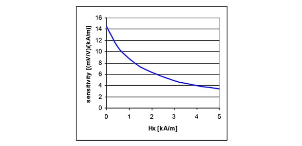
In some applications a high sensitivity is desired. In this case it is possible to work without a bias field. To do so, the sensor must be well preconditioned: immediately before the measurement, the magnetization is flipped by a short magnetic pulse in a defined x-direction (premagnetisation). To prevent the stripe magnetization of flipping during the time between premagnetisation and measurement, external fields must be limited to approx. less than 0.5 kA/m.
| Bias Field Hx in kA/m |
Operating Field Range in kA/m |
Sensitivity S in mV/V/kA/m | Max Field Hy,max in kA/M |
Remark |
| 0 | 0.35 | 14 | 0.5 | Premagnetization necessary |
| 1 | 0.5 | 10.5 | 0.5 | Premagnetization necessary |
| 2 | 1.1 | 6.3 | 1 | Premagnetization recommended |
| 3 | 1.4 | 4.9 | ∞ | Stable |
| 5 | 2 | 3.4 | ∞ | Stable |
Table 2: Sensitivity and recommended operating area.
Permanent Magnets and Barber Pole Sensors
The stabilizing Hx-field is usually generated by a permanent magnet. Using KMY20S or KMZ20S the customer has to apply a permanent magnet to generate the required bias field. KMY20M and KMZ20M are provided with an internal hard ferrite-magnet. The maximum external field strength is only limited by the stability of the permanent magnet material. In the case of the KMY20M and KMZ20M-types disturbing fields higher than approx. 40 kA/m (500 Gauss) can change the magnetization direction of the permanent magnet irreversible. This can lead to a permanent change in the offset voltage and to a destruction of the sensor function. This limitation can be extended by use of S-type sensors in combination with other magnets, like for example rare earth magnets, which have to be provided by the user.
Temperature
Both ohmic and magnetoresistance originate from scattering processes of the conducting electrons. As all scatter processes are temperature dependent, the bridge resistance and MR effect ∆R/R show a temperature dependence as well. Temperature coefficients are usually related to two temperatures via:
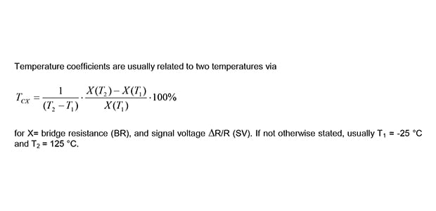
In case of Permalloy both bridge resistant and amplitude temperature coefficient have roughly the same value, but differ in sign TCBR≈-TCSV.
This fact enables the user to compensate the temperature dependence of sensitivity by using constant current supply. In this case the supply voltage increases with increasing temperature and increasing bridge resistance. This effect causes an increasing output voltage, which compensates the loss in sensitivity.
Another important value is the temperature coefficient of the offset. This temperature coefficient is caused by small differences in the temperature behavior of the four bridge resistors. In practice, a drift in the output voltage is observed, which can not be separated from the regular output signal caused by magnetic fields. In applications using DC-signal coupling the temperature coefficient of the offset will thus limit the measurement accuracy.
Permalloy is a very robust material that can withstand very high temperatures up to approx. 300°C when protected by a coating. In this case, packaging will be the limiting factor.
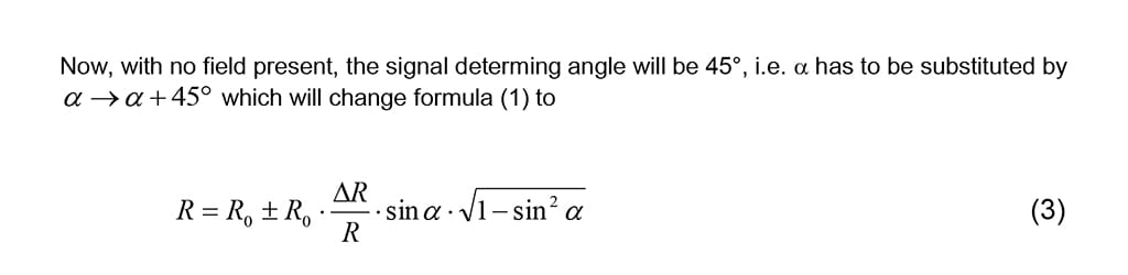
Andreas Voss presents details on magnetoresistive sensor technology and where the sensor technology can be applied.